On the challenges of predicting microscopic dynamics of online conversations

Summary

What was done?

We propose a generative model for predicting the size and structure of conversation trees on social media, which first predicts the final size of the tree and then iteratively adds nodes to the tree until it reaches the predicted size.

What was learned?

[The] model outperforms the random baseline and is competitive with the state-of-the-art CTPM Cascade Tree Prediction Model
Krohn R, Weninger T (2019) Modelling online comment threads from their start. In: Proceedings of 2019 IEEE international conference on Big Data (Big Data), pp 820–829 baseline in predicting macroscopic features such as depth, breadth, and structural virality of conversation trees. Nevertheless, the present evaluation reveals that our microscopic predictions deviate significantly from the empirical conversations. This negative result highlights the challenges of the microscopic prediction task for cascade trees: we are using a rich feature set and a strong model, and yet still failing.

Research Problem

The authors are attempting to tackle an extremely difficult task: accurately generating both macroscopic (e.g., the size and structure) as well as microscopic (e.g., the precise longitudinal evolution) properties of social media cascades.

They are attempting to do this by taking a generative approach using only the first \(k\) nodes, in some cases beginning with only the root.

As a result, the authors call their model the Tree Growth Model (TGM).

Within the Related work portion of the paper:

Generative approaches aim at identifying underlying mechanisms that can reproduce stylized traits of cascades. Aragón et al. (2017) Aragón, P., Gómez, V., García, D. et al. Generative models of online discussion threads: state of the art and research challenges. J Internet Serv Appl 8, 15 (2017). published an extensive survey of approaches of this kind.

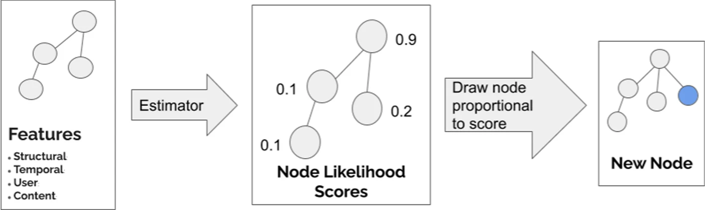
The general idea here is that the model will take two steps:

1. Size prediction: Predict the size of the complete cascade
2. Node placement: Iteratively attach nodes to the existing cascade until the number of nodes in the cascade equals the predicted size

Size Prediction

Regression is utilized to predict the size of the cascade based on the features taken from the initial \(k\) nodes.

Since regression is tough with such broad distributions (see above), they instead predict the size-quantile of the tree and then map that quantile back to a size using the empirical distribution. Several regression models were evaluated and, ultimately, a Random Forest model was selected.

Node Placement

The general idea for the node placement procedure is as follows:

To predict where the next node will be attached, we train an estimator to assign a likelihood score to each node in the current tree. We then draw a random node with probability proportional to its score. The selected node becomes the parent to the newly attached node.

Features are taken from the existing tree and each individual node. Again, various machine learning models are considered and, ultimately, a Gradient Boosting Tree classifier was selected as it performed best.

The raw classifier scores did not return great results so they applied a Bayesian See the Node placement section for details on this correction correction to the raw classifier output to obtain each node's likelihood estimate (of being selected as the new node's parent).

See below for a graphic of the above described two step process...

Baseline models

The authors provide a wonderful overview of the different baselines utilized in the study.

Random baseline

A random size baseline model draws a random size for each prediction from the empirical distribution of sizes with replacement. We then use a simple random choice baseline for node placement, in which all nodes are equally likely to receive the next reply. Let \(j\) be the time-ordered index of existing nodes, and let n be the number of existing nodes in the tree. The probability of node \(x_j\) being the parent of the next node is given by \(P(x_j)=\frac{1}{n}\).

CTPM baseline

The Cascade Tree Prediction Model uses Hawkes processes to reconstruct the structure of the cascade tree. While the details are found elsewhere (Krohn and Weninger 2019), here we explain the intuition behind the approach. Two distributions are fit, one for the root node and one for the other nodes, which determine branching factors at each node. CTPM infers the parameters of these distributions for each test post from similar posts in the training set. For each node, the number of children is drawn from its distribution, and the tree is constructed in a breadth-first way. The size is implicitly determined when the branching process stops after leaf nodes draw zero values for their numbers of children.

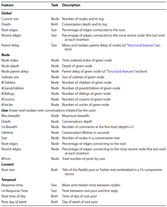
Feature description

The final TGM model utilizes four classes of features:

1. structural
2. user
3. content
4. temporal

The vast majority of features are straight forward and, thus, I refer the reader to the original text for more details. Nonetheless, below I include a table from the paper which summarizes the authors include.

However, the authors also introduce a novel metric (parent delay) discussed directly below.

Parent delay

More formally, this metric is called the normalized delay steps since parent measure. Which the authors describe in the following way:

It is an edge attribute capturing the relative difference in steps (actions) between a new node and its parent. Let the index node \(i\) be ordered by the time of creation of the node. Then the parent delay of node \(i\), \(d_i\), is given by: $$d_i = \frac{ (i - \pi(i)) - 1 }{ i - 1 }$$ where \(\pi \left(i\right)\) is \(i\)'s parent ( \(i > \pi \left(i\right)\) ) and \(d_i \in \left[0,1 \right] \). The root index is 0, so the parent delay of the second node attached to the tree is undefined. That is, \(d_i\) is defined only for the second edge (third node) and on. This measure aims to capture the root bias and the novelty features in prior work See the Structural features section for references to this prior work . When a node is connected to the root, this edge is the most delayed possible [and] \(d_i = 1\). Conversely, attaching a node to the most recent node previously added to the tree gives the shortest delay [and] \(d_i = 0\).

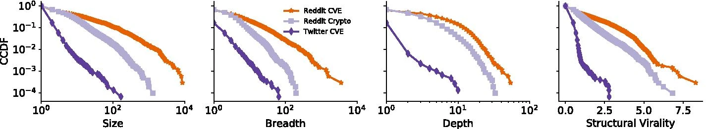
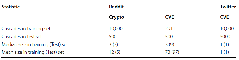
Datasets

Three (non-public) datasets - provided as part of the DARPA SocialSim December 2018 Challenge - were utilized for testing the TGM. Two originate from Reddit and a third from Twitter.

Both platforms contain Common Vulnerabilities and Exposure (CVE) codes It is not clear what this means/represents. I could not find details about this in the article or it's appendix. and related keywords. These make up two of the three datasets while the third is related to cryptocurrency discussions on Reddit.

All models were tested based on a cross-validation hold-out procedure where some data is used for training and the remaining portion is used for testing. Below is a table illustrating the size of each dataset's training/testing split.

Evaluation

The model was evaluated for each sub-task (i.e., size prediction and node placement), as well as the overall combined task of predicting the cascade size and structure of the whole conversation trees.

Below I summarize the evaluation metrics.

Size Prediction

For the size prediction task, Relative Error is used as their metric. It is calculated as \( \frac{|s - \hat{s}|}{|s|} \), where \(s\) is the true size and \( \hat{s} \) is the estimated size of the tree.

Mean Relative Error (MRE) across all trees is reported.

Node placement

Node placement is evaluated by seeing whether or not the TGM does better than the random choice baseline model.

In the baseline model, if there are \(n\) nodes in a tree, the probability of selecting the correct parent node, \(i_{n}^{*}\), when attaching a new node is \(P(i_{n}^{*}) \).

To compare the models more easily, the mean probabilities are normalized by the baseline model. This metric is called the Relative Performance of the next-node placement task.

Whole-tree simulation

This task is evaluated using macroscopic measures of tree structure:

• depth
• breadth
• structural virality (Wiener index) - average distance between all pairs of nodes in the tree

Results

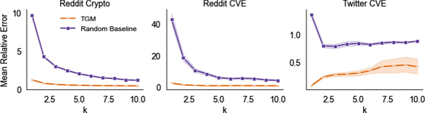
Size prediction

For Reddit, the authors find that error decreases as the number of initial nodes ( \(k\) ) increases because the regressor has more information. However, for Twitter they find that performance decreases as \(k\) increases.

As explained by the authors:

We attribute this to training data sparsity. As \(k\) increases, the number of potential targets for new nodes increases while the number of examples decreases: there are far fewer Twitter cascades of size 10 than of size 2. Consequently, the regression model has too few examples to learn from, and the random baseline model fails to adapt to the change in initial tree size.

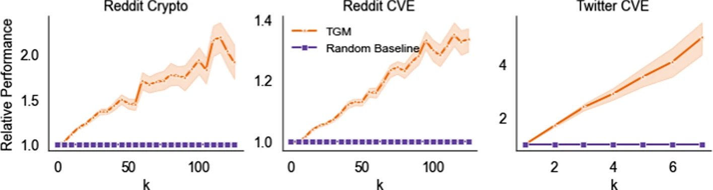
Node placement

The TGM model substantially improved node performance relative to the random choice baseline (see below).

Whole-tree simulation

The plot in this section reflect performance based on the amount of initial information provided - i.e., based on the size of \(k\). TGM outperforms the random baseline model of all tested values of \(k\) on the Reddit datasets but struggled with larger \(k\) values in the Twitter dataset.

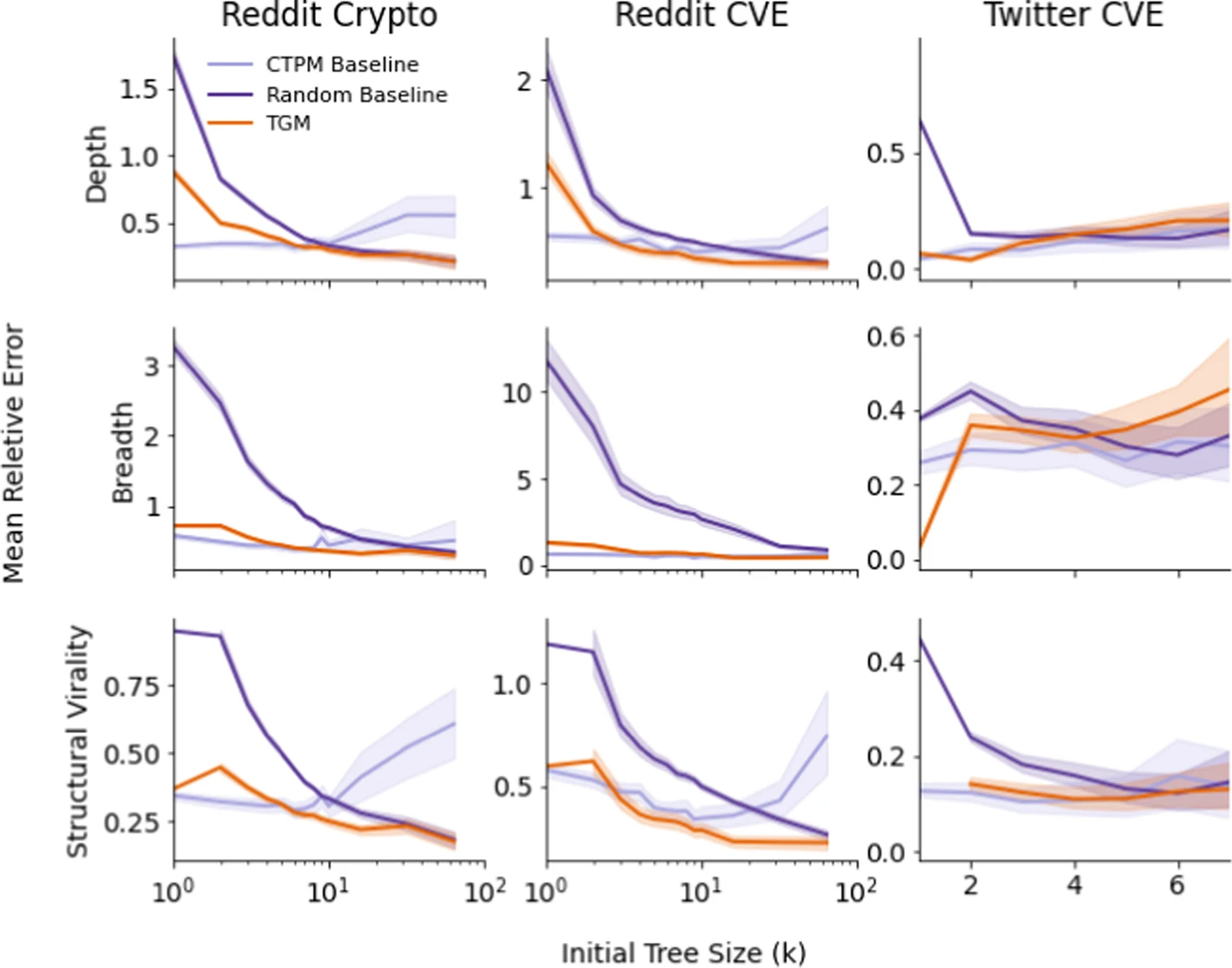
The authors believe this again may be due to data sparsity:

This may be due to data sparsity; only about 1% of the tress in the training set have size larger than 5.

However, the authors also look at how performance varies based on the size of the final tree in the below figure.

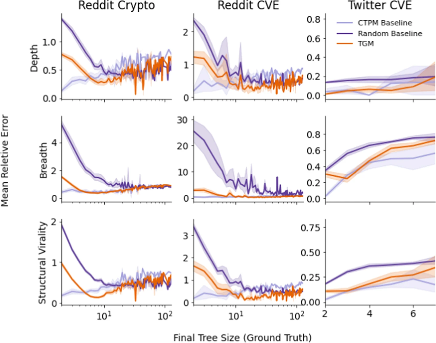
In this case, the authors find that:

• the model generally outperforms the random baseline
• it performs best for smaller trees (more data)
• converges to random baseline error for larger trees (less data)
• the CTPM does better on small Reddit trees but the TGM does better for medium/large trees
• CTPM performance is comparable to TGM on the Twitter dataset

Cumulative node placement

The model does well with respect to predicting macroscopic structure of a cascade - but how does it predict microscopic structure?

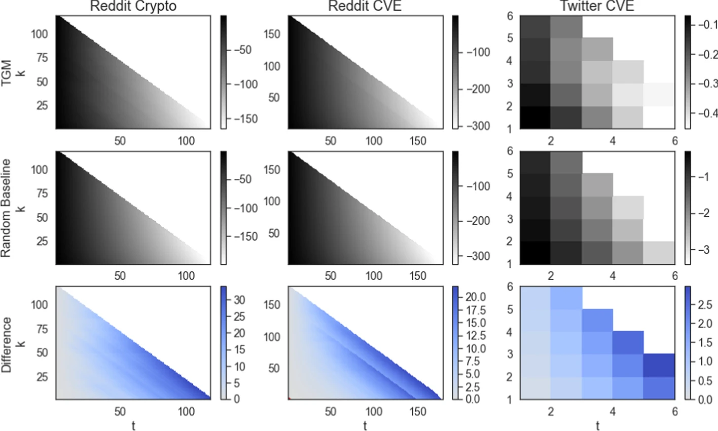
Here is how the authors describe the above figure/results:

... our model outperforms the baseline in consecutive node placement on all datasets and all values \(t\) and \(k\); the difference is very small for very small \(t\) (short prediction sequences). However, the small values of the log-probabilities indicate that the model is very rarely capable of correctly reproducing the microscopic evolution of the conversation trees, especially for long node placement sequences (large \(t\)). ... We believe that this poor performance is due to the accumulation of errors: even if we have a decent chance of selecting the next node correctly, the odds of doing so many times in a row drop geometrically.

An interesting point from the article on micro versus macro performance differences...

How can our model do so poorly at microscopic predictions far into the future, and yet do reasonably well in predicting the structure of the final trees? This apparent contradiction reveals a lack of sensitivity of the traditional structural measurements. When a tree has many nodes, there are many distinct microscopic configurations leading to almost identical macroscopic structural properties such as size, depth, breadth, and structural virality. In other words, predicting these structural features is a lot easier than reproducing the evolving conversations.